Overview

Blending two superimposed images can be done in many ways. As I have shown before, tricks such as alpha blending and multiresolution blending can be used to achieve this. Now I want to demonstrate a more powerful technique: Poisson Blending. While the previously two mentioned techniques work with the spatial domain and frequency domain respectively, Poisson blending deals with the gradient domain.

Let's look at some results and see how it works...

Toy Problem

As a simple warm up we first test gradient domain processing implementation on a toy example. Using the given toy image, we set up and solve a least squares problem such that:

The x and y gradients of our new image closely match those of the original.
The top left corners of the two images should be the same color.

Here is the result:

Original	Solution	Difference

As you can see, the solution to the least squared problem is, correctly so, identical to the original. It only makes sense that the image with gradients closest to the original image and top left corner the same color as the original image is the orignal image itself.

Let's dive deeper into the process and see the results on more interesting input images...

Poisson Blending

Let us call the image to be superimposed on to the other the source image. The image that the source will be overlayed on will be the target image. The idea is to find the right pixel values such that the gradients of the target and where the source will be are the most consistent. We can represent each pixel as a variable and the problem then boils down to solving a system of linear equations such that the gradients of the new pixels match the gradient of the original image. Of course there is not a perfect answer so we can instead set the problem up as a least squares problem. To illustrate the process more mathematically, we are trying to find the following:

Where v is the pixel-vector representing the calculated values to use to represent the blended superimposed image, s is the pixel vector representing the source image, t is the pixel vector representing the target image, and N is the set of 4-neighbor pixels ( the pixels above, below, and on each side of v[i] ).

Here is my favorite result:

Source	Target	Unblended	Blended

And here are some more results...

Source	Target	Unblended	Blended

While the above results worked well for the most part, not all of the images I tried came out well. For example let's look at the following:

Source	Target	Unblended	Blended

As you can see the results are not that great. The first image shows that poisson blending still has the drawback that nearly all blending techniques do in that the images must be carefully aligned before blending to prevent artifacts or irregularities that expose the blend. The second image shows another problem. In order for the image to look realistic, the texture from the bricks should still show through the mona lisa yet they do not. There is a variant technique that will fix this though...

Mixed Gradients

Mixed Gradient blending is very similar to Possion blending with one small but important difference that is first best shown with the mathematical equation:

Note the difference. In the original equation we aimed to make our new images gradients closest to the source images gradients, except when on the border of the source image where we aimed to make the gradient of the new image and the target image closest to the gradient of the source image.

With mixed gradient blending, however, instead of always comparing to the source image gradient, we compare to d[i,j], which is defined as the value of the gradient from the source image or the target image, whichever has the larger magnitude.

Let's see some results:

Source	Target	Unblended	Blended

Comparing the Different Blending Techniques

We have now dealt with a range of blending techniques. Let's see how they all compare:

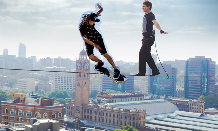
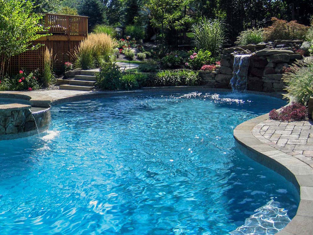
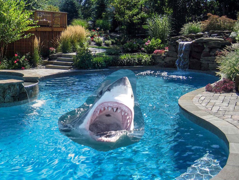
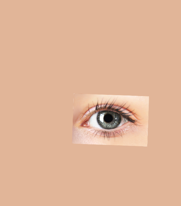
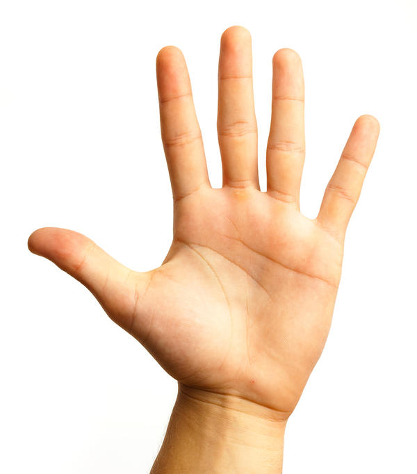
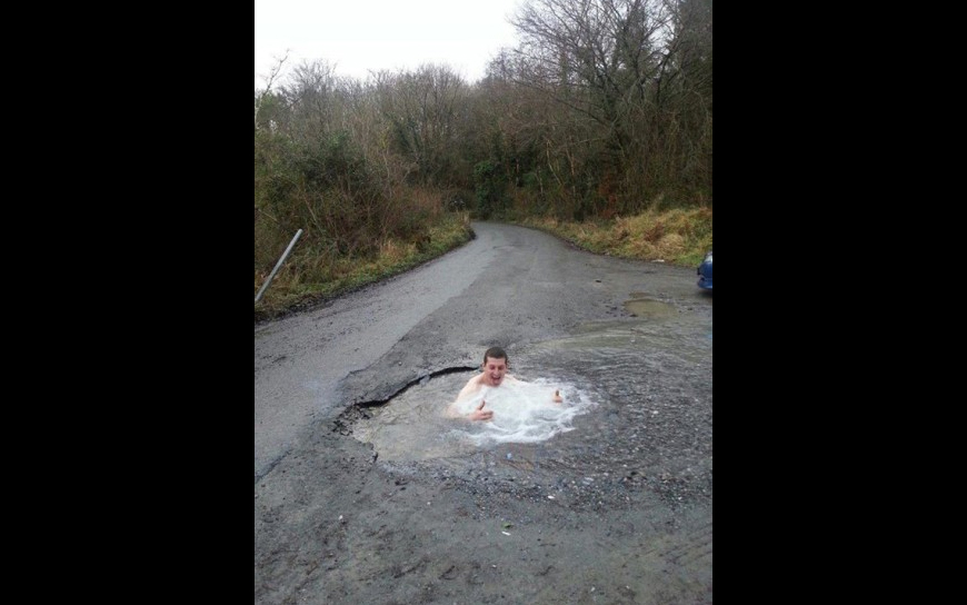
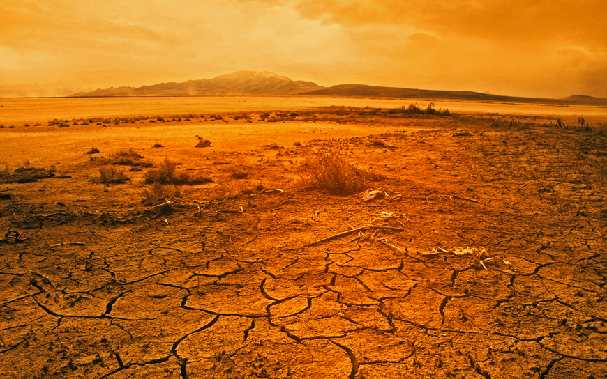
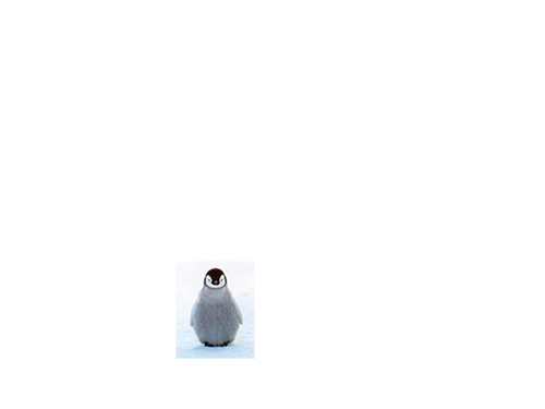
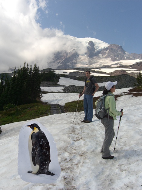
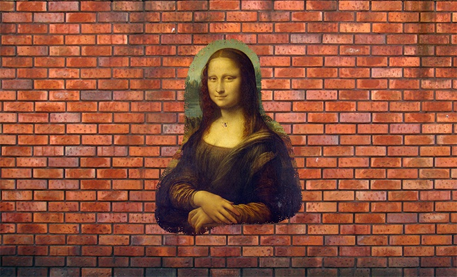
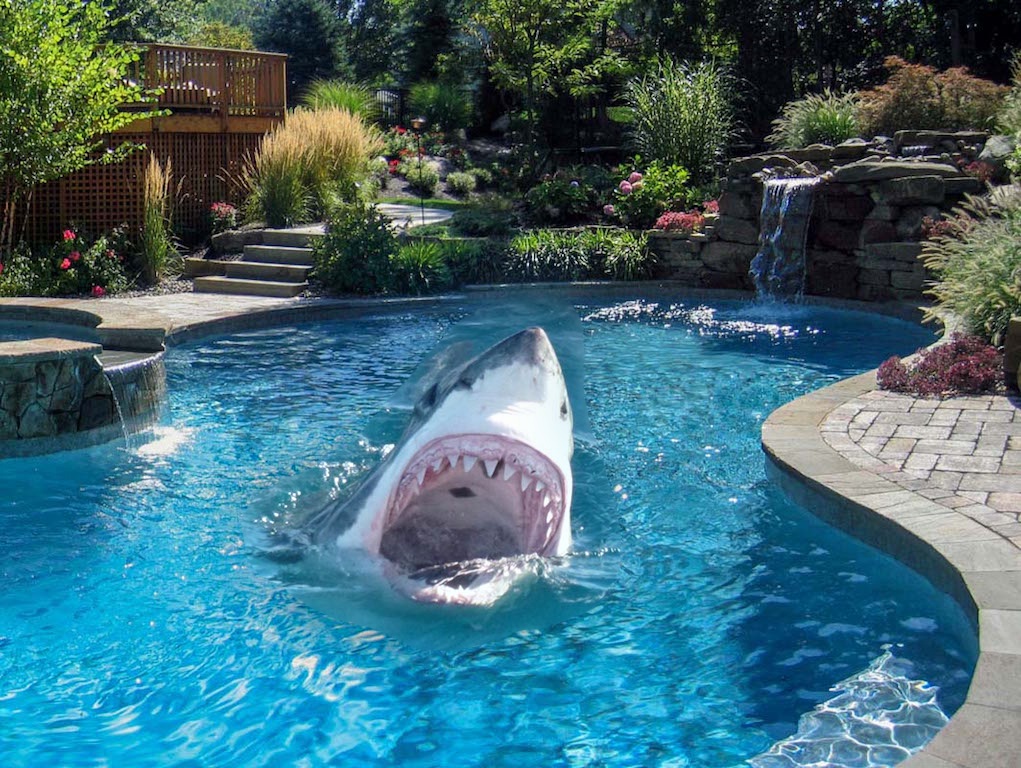
Here is the image we will use to compare:

Source	Target	Unblended

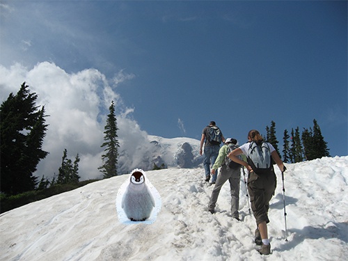
And here are the results from the three different blending techinques:


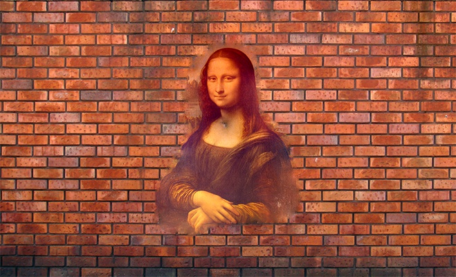
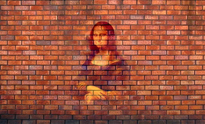
Multiresolution (Laplacian)	Mixed-Gradient	Poisson

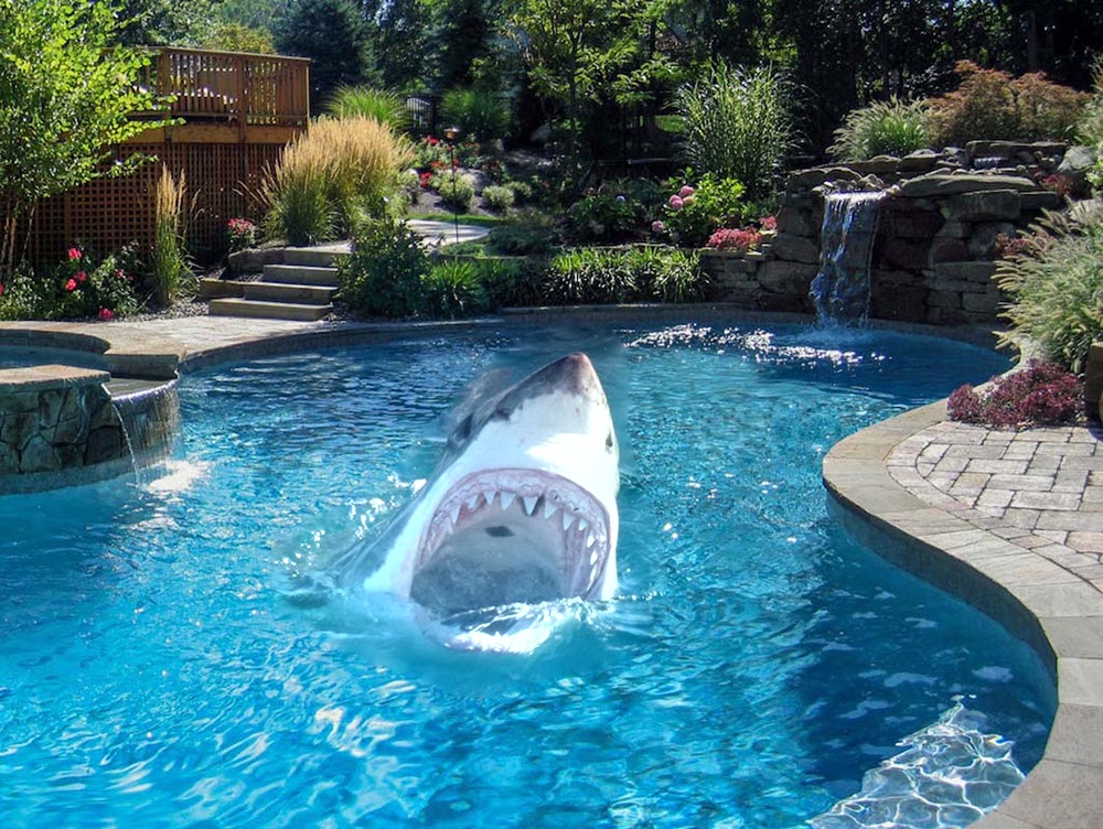
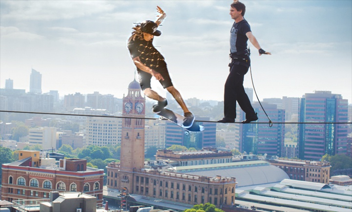
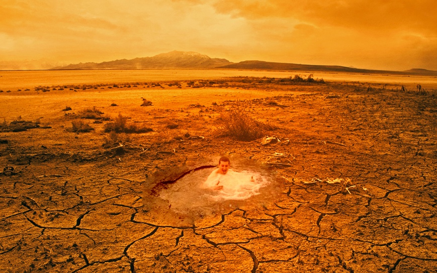
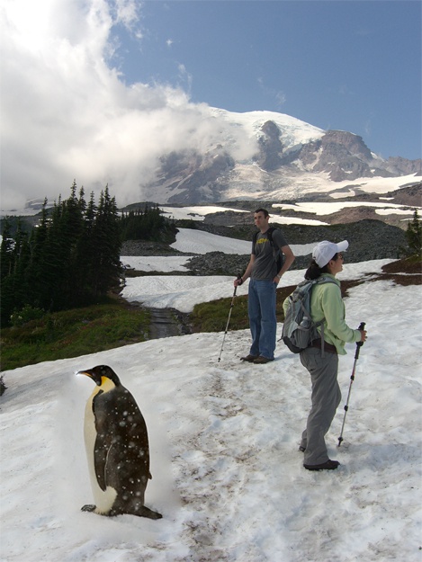
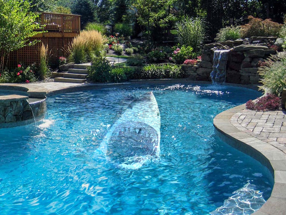
In this case, and it may not always be the case, Poisson blending seems to be the top performer.

The multiresolution blending does a good job of hiding the sharp edge between the two images that can be seen in the unblended image. However, multiresolution blending can do nothing about the color of the images, so the color difference between the water from the pool and the ocean remains and this creates an undesirable image.

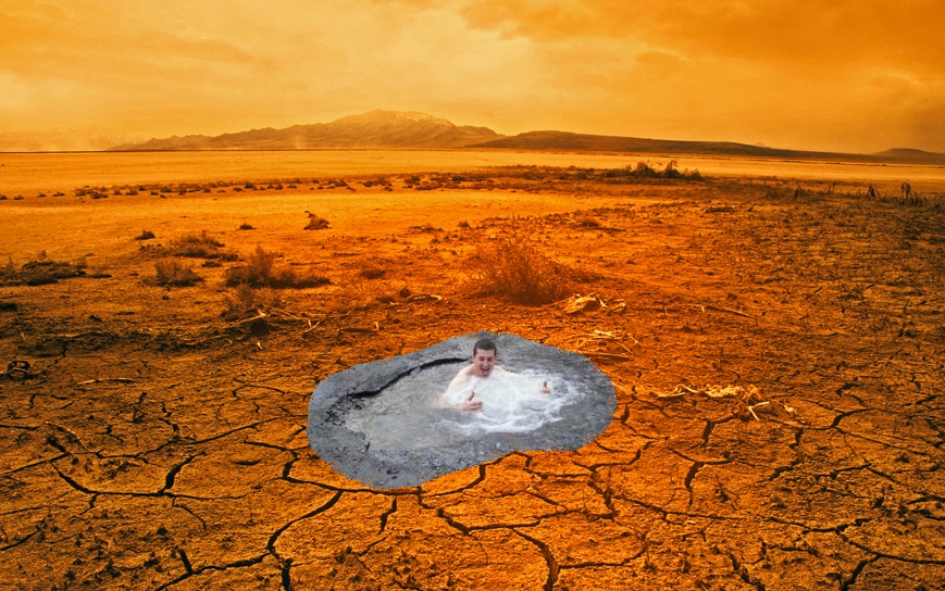
The mixed-gradient blending does a better job matching the colors of the waters. However, as you can see, the shark becomes unrealistically transparent. This is due to the nature of how we calculate the mixed-gradient pixels. Recall that we used the gradient from the source image or target image that was larger in magnitude. Notice that the ripples in the water of the target image form sharp edges. These will result in many large magnitude gradients and so we more often attempt to make our shark blend in with the target image, resulting in the alpha effect.

This is why, in this case, the Poisson seems to be the best happy medium. The Poisson blending does a great job of matching the water colors, and while this does cause the sharks color to be changed as well, it is not changed so much that is is transparent and unrealistic.

I suppose each method has its strengths and ideal conditions however, and so there is no one method that always produces better results for every pair of images.

Color2Gray

When converting color images to grayscale using standard techniques such as the rgb2gray function does, you may lose some important information that was encoded in the colors. Perhaps now, equipped with the power of gradient domain processing, we can do better.

What we want is a grayscale image that has similar contrast to its color counter part. Achieving this with poisson blending is quite simple.

We first convert the image to the HSV coordinate system. Recall that HSV encodes images in terms of Hue, Saturation, and Value. In this coordinate system we can immediately examine an images color, the intensity of that color, and the brightness.
We then use Poisson blending to "blend" the H and V channels of the image. This essentially takes the image representing brightnesses, which is similar to the rgb2gray version, and tweaks the gradients so they match the gradients of the hue channel. The result is a grayscale image that experiences change whenever there is a color change in the original image.

From this we get a much more informative grayscale image, as shown below:

Original	Using rgb2gray	Using gradient domain processing