Fluid Simulation

Christine Zheng, Gus Silva

Abstract

In this project we explore a tricky subject: simulating the movements of fluids. We first develop a simple particle renderer with controls. We then attempt to use a particle-based approach to simulate water. The key to simulating any fluid is enforcing incompressibility. Unfortunately, this is computationally expensive. In the paper Position Based Fluids, Muller and Macklin describe a method for simulating fluids in a relatively efficient manner while not requiring impractical timesteps. We attempt to implement the various ideas in this paper such as enforcing incompressibility by incorporating density constraints into Position Based Dynamics, simulating surface tension by adding artificial pressure, and reducing damping by adding vorticity confinement and viscosity.

Technical Approach

Particle Renderer

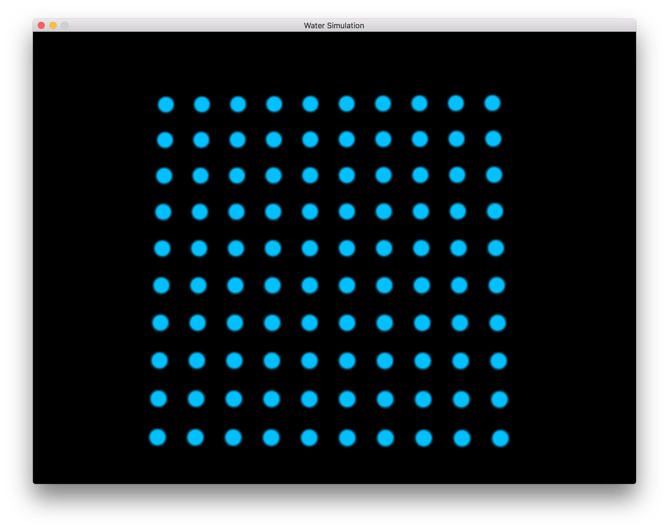
Before we could simulate anything, we needed something to view our results on. We followed the excellent tutorials on opengl-tutorial.org and learned how to use openGL to create a window and render objects. We then tailored this to our need in order to render our particles that would eventually simulate water.

Basic Particle Renderer

Controls

We now wanted a way to navigate our space. Thankfully, the GLFW Library provides plenty of functions to get user input. We decided to go with FPS like controls and so the arrow keys allow the camera to strafe in the respective direction and moving the mouse affects the direction in which the camera is pointed. We now have a convenient way of viewing our particles from any point of view that we like.

Controls in action

Water Simulation

Now that we have a basic particle renderer and a way to navigate, let's add some action to our particles!

Pseudocode

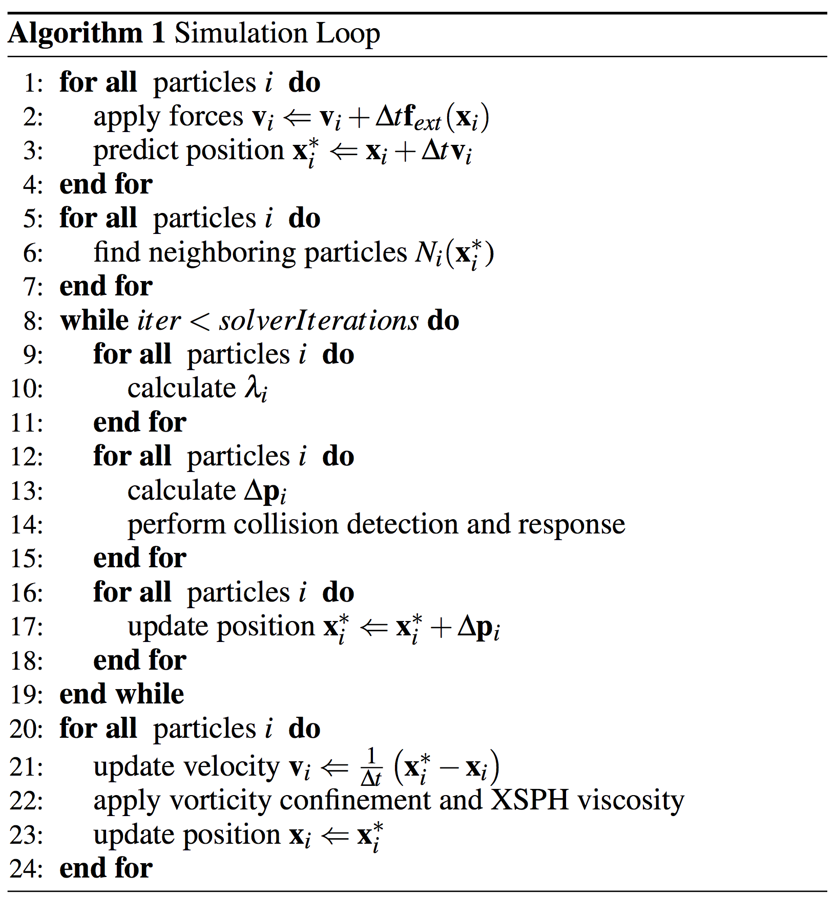
As previously mentioned, we follow the technique described by Macklin and Muller in the Position Based Fluids Paper (linked above). From a high level, the algorithm is as follows:

PBF Pseudocode

Predict Positions and Apply Forces

The first part of nearly any physically based simulation is of course to apply external forces. For this part the only external forces acting on our particles is gravity. We then do the classic update of the velocity as v = v + a * deltaT and update position as x = x + v * deltaT. We used a constant deltaT of 1/60. This caused the real time rendering, of course, to be out of sync and look unrealistic. In order to achieve the realistic time we simply output an image each time step and then create a video from these images with 60 FPS.

Here is our simulation so far with just external forces applied:

Particles falling due to gravity

Finding Neighbors

The next step in the algorithm is to find a particles neighbors. In order to do this, we implement a similar technique to the one in our cloth simulation. We first divide our space into an evenly spaced grid. We decided to break the space into boxes with width, height, and depth equal to 1.5 times the radius of our particles. We then hash each particle based on which box it falls into. One key difference from the cloth simulation is that instead of considering only particles in the same box neighbors, we search the 27 surrounding boxes for neighbors as well. This is because we would like a more accurate count of neighbors so we can get a more accurate estimation of density in the next part. Thus we go through all the boxes mentioned above and add a particle j to particle i's list of neighbors if j is within radius*1.5 of i.

Below we visualize one particles neighbors. The particle we are looking at is in red, and its neighbors are white.

VIsualization of Neighbors

Enforcing Incompressibility

The main bulk of simulating fluids, and thus the main bulk of the paper, is maintaining constant density, or enforcing incompressibility. In other words, for each time step, we want to move the particles such that the density around each particle is as close to the rest density as possible.

Obviously, the first thing we need is a way to estimate the density. Now that we have each particles' neighbors, this can be done using the SPH Density estimator. We define the density for the ith particle as:

$$\rho_i = \sum_j m_j W(p_i - p_j, h)$$

Where $W(r,h)$ is a smoothing kernel. To be consistent with the paper we used the Poly6 Kernel for the non-gradient calculations and the Spiky Kernel for the gradient calculations. One small note is that we give all particles an equal mass so we drop the $m_j$ term in the above calculation.

We can now express our desire for a constant density as a mathematical constraint. Thus, we define a constraint function for each particle, where the constraint for the ith particle is:

$$C_i(p_1, .., p_n) = \frac{\rho_i}{\rho_0} - 1$$

Where $\rho_0$ is the rest density and $p_1, ..., p_n$ denotes the position of the ith particle and all of its neighbors.

A Quick Aside On Position Based Dynamics

As was previously mentioned, Particle Based Fluids works by incorporating the density constraint into the Particle Based Dynamics method. PBD works by looking for a correction to the positions such that the constraint function is zero. In other words, PBD seeks a $\Delta p$ such that:

$$ C(p + \Delta p) = 0 $$ It does so by a series of Newton steps along the constraint gradient. In other words: $$ \Delta p \approx \nabla C(p)\lambda $$ $$ C(p + \Delta p) \approx C(p) + \nabla C^T \Delta p = 0 $$ $$ C(p + \Delta p) \approx C(p) + \nabla C^T \nabla C(p) \lambda = 0 $$ $$ \lambda = - C(p)(\nabla C^T \nabla C(p))^{-1} $$

Back to Position Based Fluids

For position based fluids, we simply use our density constraint function as $C$ and get: $$ \lambda_i = - \frac{C(p_1, ..., p_n)}{\sum_k |\nabla_{p_k} C_i|^2} $$ In order to prevent numerical instability in the denominator, we use Constraint Force Mixing, which mixes some of the constraint force back in to the constraint. The result ends up being that we add some constant value $\epsilon$ to the denominator and so our final lambda calculation for the ith particle becomes: $$ \lambda_i = - \frac{C(p_1, ..., p_n)}{\sum_k |\nabla_{p_k} C_i|^2 + \epsilon} $$

Now recall that $\Delta p = \nabla C(p) \lambda$. We have now solved for everything we need to in order to calculate $\Delta p$, which is the change in postition such that the constraint function equals zero. In our case, this means we now can calulate the change in each particle's position such that its density is about the same as our rest density! For each particle i, the total number of corrections is:

$$ \Delta p_i = \frac{1}{\rho0} \sum_j (\lambda_i + \lambda_j) \nabla W(p_i - p_j, h) $$

At this point, using the above position update rule we ge the following:

Update Velocity with Vorticity Confinement and XSPH Viscosity

In the above video, we get good results, but the movement is very dampened. This is a side effect of using Position Based Dynamics. One way to fix this is to increase the number of iterations but this quickly becomes unreasonable. A better solution is the one used in the Position Based Fluids paper which is to add vorticity confinement and viscosity to our simulation.

Vorticity is the measurement of spin and rotation in a fluid. It can be observed by watching particles' relative displacements when they move along the flow. We added the vorticity by applying a corrective force. We estimated the vorticity of a particle followed by the equation from the paper:

$$ w_i = \sum_j v_{ij} \times \nabla_{p_j} W(p_i - p_j, h) $$ where $$ v_{ij} = v_j - v_i $$ the difference between the current particle's velocity and the velocity of its neighbor particles. We can then calculate the corrective force using below equation: $$ f^{vorticity}_i = \epsilon (N \times w_i) $$ where $N$ is: $$ N = \frac{\nabla_{|w|_i}}{|\nabla_{|w|_i}|} $$

We also apply viscosity to our water to reflect the "thickness" of the fluid. Similar to the shearing force from the cloth simulation, fluid also have shearing force. Viscosity is the force which fluid resists that distortion. Thick fluid has high viscosity, thin fluid like water has low viscosity. So water particles appear to not stick compared to oil particles. We can do so by updating the particle's velocity as:

$$ v^{new}_i = v_i + c \sum_j v_{ij} * W(p_i - p_j, h) $$

Adding the vorticity confinement and viscocity to our simulation gives us the following:

As we can see, the fluid is much more...fluid. Less damping occurs, we get nicer splashes, and the fluid rebounds and "sloshes" in a manner more similar to real water.

Improving visuals with "foam"

We originally had all the particles appear as blue. We think it is better to have the particles with higher velocity to appear in whiter colors so the fluid looks more like foam. In order to change the particles' colors according to their velocities. We followed the equation from the original report:

$$ c = 1 - (\frac{1}{v^2_x + v^2_y + v^2_z})^2 $$ $c$ represents the whiteness of the particles' color. So the higher the velocity, the bigger the c is. We maintain c as a positive value by capping it between 0 and 1. We used HSL to get the updated color and converted it back to RGB and applied it to the particles.

This was the last touch and we now get our final result:

Final Result

Problems Encountered and Lessons Learned

Timing is everything. In an effort to lock our simulation in with real time, we originally calculated $\Delta t$ each iteration using the true difference in time since the last iteration. Early on this seemed fine. However, as our simulation grew more complex we began getting strange results. We eventually realized, after visiting office hours (thanks Kevin!), that our timestep was too small and this was causing problems. We changed our $\Delta t$ to a constant 1/60 and things returned to normal.
Small tweaks in parameters can make a huge difference. As one can see, this simulation method has many tweakable parameters. Lambda relaxation parameter, rest density, particle radius, vorticity epsilon, viscosity constant, etc. We originally underestimated how important these parameters were and so after we initially implemented the algorithm we were not getting good results. Again, after visiting OH we were told that these parameters were important and we should spend time carefully tweaking them to perfection. In doing this we realized how important and sensitive they were. For example, a change of 0.1 in the vorticity epsilon could make the difference between a great simulation and a completely out of control one.

Contributions

Christine Zheng

- Controls, Applying Forces, Viscocity Confinement, Vorticity

Gustavo Silva

- Particle renderer, Finding Neighbors, Enforcing Incompressibility, Improving Visuals